PythonのStatsmodelsを使って回帰分析を行う
Pythonを使って回帰分析を行う。使用するライブラリはStatsmodelsである。
In [78]:
%matplotlib inline
まず対象となるデータを読み込む。これはR処理系に付属しているattitudeというデータを write.csv(attitude, "attitude.csv", quote=FALSE, row.names=FALSE) でCSVにしたものである。
この記事を書くにあたって参考にしている「定性的データ分析」(金明哲)によると、 このデータは35人の事務員に対するアンケート結果で、それぞれの列は次のような意味である。 (ところどころ意味が分からないのだが)
rating: 総合評価, complaints: 従業員の苦情の取り扱い, privileges: 特権は許さない, learning: 学習の機会, raises: 能力に基づいた昇給 , critical: 加重, advance: 昇進
まずは散布図行列を描く。
In [80]:
from pandas.tools.plotting import scatter_matrix
scatter_matrix(attitude, figsize=(7, 7))
plt.show()

数字は満足度の割合(パーセンテージ)である。総合評価ratingとcomplaintsに相関が高そうだということが見て取れる。 対角線上にはその列(行といっても同じだが)の変数のヒストグラムが表示される。
次にStatsmodelsを使い、ratingを目的変数、残りのすべてを説明変数として重回帰分析を行う。 add_constantという関数は1という値だけの列を追加していて、これが切片(説明変数にかかわらずオフセットされる量)となる。 Statsmodelsの流儀で、モデルに切片を使う場合はこのようにしなければならない。
In [81]:
import statsmodels.api as sm

# Fit and summarize OLS model
y = attitude['rating']
X = attitude[['complaints', 'privileges', 'learning', 'raises', 'critical', 'advance']]
mod = sm.OLS(y, sm.add_constant(X))
res = mod.fit()
print res.summary()
この結果が妥当だとすると、回帰係数coefにより、complaintsやlearningが大きいほど総合評価ratingは上がる。逆にadvanceが高いほど総合評価は下がるということになるようだ。
回帰モデルの評価指標としてサマリーの右上に表示されているような指標値がある。
Log-LikelihoodとR-squaredはモデル作成に使ったデータへの当てはまりの良さを示す。 しかし一般的に説明変数が多いほどデータへの当てはまりは向上するが、それが未知のデータの予測に良いとは限らず、これらの値が高くても無駄な変数を含むかもしれない。 AICやAdj. R-squaredは当てはまりの良さを説明変数の数で打ち消すような効果を持つ。
回帰変数に対して表示されているP>|t|は回帰変数に対してt検定を行った場合のp値であり、小さいほどその変数の影響が偶然でない可能性が高い (検定を行う場合は0.05未満や0.01未満が基準となる)。 そこで、P>|t|の小さい順に変数を追加していって、評価指標がどのように変化するかを見てみる。 ここでは変数を追加していくコードを自分で書いているが、おそらく自動で行うような関数もあるのかもしれない。
In [82]:
def olc(i):
    y = attitude['rating']
    X_labels = ['complaints', 'learning', 'advance', 'privileges', 'raises', 'critical'][0:i+1]
    X = attitude[X_labels]
    mod = sm.OLS(y, sm.add_constant(X))
    res = mod.fit()
    return [res.llf, res.aic, res.rsquared, res.rsquared_adj, X_labels]

DataFrame(
    [olc(i) for i in range(0, 6)],
    columns=['Log-Likelihood', 'AIC', 'R-squared', 'Adj. R-squared', 'vars'])
Out[82]:
Log-LikelihoodとAdj. R-squared(いずれも高いほうが良い)は変数を増やすのにつれて単調増加している。
一方AIC(低いほど良い)とAdj. R-squared(高いほうが良い)は向上が頭打ちになるポイントがある。 AICの場合[complaints, learning]を説明変数に使ったときが最もよく、Adj. R-squaredの場合[complaints, learning, advance]を使ったときが最もよい。
なおAICの値は「定性的データ分析」のRの実行結果に出てくる値とは一致しておらず、何か計算方法に違いがあるのかもしれない。
AICをもとにすると[complaints, learning]だけを説明変数にするのがよいようだ。改めてサマリーを生成したものを次に示す。
In [83]:
# Fit and summarize OLS model
y = attitude['rating']
X = attitude[['complaints', 'learning']]
mod = sm.OLS(y, sm.add_constant(X))
res = mod.fit()
print res.summary()
In [84]:
import statsmodels.formula.api as smf

mod = smf.ols(formula="rating ~ complaints + learning", data=attitude)
res = mod.fit()
print res.summary()
回帰分析では説明変数同士の強い相関によって回帰モデルに矛盾が生じることがある。 これをチェックする指標としてVIF (Variance Inflation Factor) という値がある。
StatsmodelsでVIFを計算する関数variance_inflation_factorは少し使いにくい形をしている。 説明変数とVIFを計算したい列の番号を引数として与える。 ここでは切片を含めてすべての列に対するVIFを計算した。
In [85]:
num_cols = mod.exog.shape[1] # 説明変数の列数
vifs = [variance_inflation_factor(mod.exog, i)
        for i in range(0, num_cols)]
DataFrame(vifs, index=mod.exog_names, columns=["VIF"])
Out[85]:
VIFの値が10より大きいときは多重共線性があるとされる。 Statsmodels の variance_inflation_factor のリファレンス では5より大きい場合となっている。 この場合 complaints も learning も1.56程度であり、多重共線性はないと判断される。切片の分はよくわからないが、切片についてVIFを計算している例をみたことがないので無視してよいのだろう。
In [ ]:
中心極限定理のシミュレーション
In [146]:
%matplotlib inline
from numpy.random import normal, poisson
import scipy.stats as stats

def show(data):
    data = Series(data)
    plt.hist(data)
    plt.show()
    print data.describe()
    print "skewness:", data.skew()
    print "kurtosis:", data.kurtosis()
    stats.probplot(data, dist="norm", plot=plt)
    plt.show()
In [147]:
data = normal(loc=16, scale=16, size=10000)
show(data)


In [148]:
def sample_and_show_means(data, num_samples=100, num_iterations=1000):
    print "Sample Distribution"
    population = Series(data)
    sample_means = []
    for i in range(0, num_iterations):
        sample_means.append(population.sample(n=num_samples).mean())
    sample_means = Series(sample_means)
    show(sample_means)
この関数はデフォルトでは標本サイズ100のサンプリングを1000回行う。これを使って先ほどの正規分布の母集団からサンプリングを行う。
In [149]:
sample_and_show_means(data)


In [150]:
sample_and_show_means(data, num_samples=16)


In [151]:
data = poisson(lam=2, size=10000)
show(data)
sample_and_show_means(data)


In [152]:
data = np.concatenate([poisson(lam=2, size=10000), normal(loc=16, scale=2, size=10000)])
show(data)
sample_and_show_means(data)


母集団のほうはなんだかよくわからない分布であるが、標本平均のほうはとにかく正規分布に従っていることがわかる。
機械学習で時間帯を説明変数にする
機械学習や多変量解析で「時間帯」(何時ごろに発生したイベントであるか)を説明変数として使いたい場合どのようにするのがよいか。
何時に発生したかというのは生データの中では0時から24時までの数値として与えられるだろう。最初に思いつくのはこれをそのまま間隔尺度として利用する方法だ。
まずは実験のための適当なデータを作る。3時、12時、24時を中心に正規分布する3つのグループのデータを生成する。
%matplotlib inline
from numpy.random import normal

num_samples = 1000

hours = [3, 12, 24]
groups =[Series(normal(size=num_samples)).add(hour).mod(24) for hour in hours]
bins = (range(0, 24))
plt.hist(groups[0], bins=bins)
plt.hist(groups[1], bins=bins)
plt.hist(groups[2], bins=bins)
(array([ 313.,  136.,   21.,    2.,    0.,    0.,    0.,    0.,    0.,
           0.,    0.,    0.,    0.,    0.,    0.,    0.,    0.,    0.,
           0.,    0.,    3.,   26.,  145.]),
 array([ 0,  1,  2,  3,  4,  5,  6,  7,  8,  9, 10, 11, 12, 13, 14, 15, 16,
        17, 18, 19, 20, 21, 22, 23]),
 <a list of 23 Patch objects>)
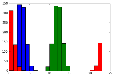
このように24時付近のグループは0時過ぎと24時前の2つに分かれる。
このデータを機械学習アルゴリズムを使って分類してみよう。 まずはデータと分類ラベルを訓練データと検証データに分ける。
from sklearn import cross_validation

X = pd.concat(groups).reshape(-1, 1)
y = pd.concat([Series([hour for _ in range(0, num_samples)]) for hour in hours])

X_train, X_test, y_train, y_test = cross_validation.train_test_split(X, y)
まずは線形分類器を使用する。
from sklearn.linear_model.perceptron import Perceptron
clf = Perceptron()
clf.fit(X_train, y_train)
clf.score(X_test, y_test)
0.22666666666666666
from sklearn.svm import LinearSVC
clf = LinearSVC().fit(X_train, y_train)
clf.score(X_test, y_test)
0.67200000000000004
線形分類器の正答率はあまり高くない。理由は比較的明白で、24時付近のグループを分類する問題が線形分離(ここでは変数が1つなので点分離というべきか)可能でないからだ。これはXOR問題と呼ばれる。
次のようにカーネル法を用いたSVMや決定木では高い正答率が出る。
from sklearn.svm import SVC
clf = SVC().fit(X_train, y_train)
clf.score(X_test, y_test)
0.95333333333333337
from sklearn.tree import DecisionTreeClassifier
clf = DecisionTreeClassifier().fit(X_train, y_train)
clf.score(X_test, y_test)
0.93333333333333335
決定木のグラフも見ておこう。
from sklearn.externals.six import StringIO
from sklearn.tree import export_graphviz
from IPython.display import Image
import pydot_ng

def draw_dt(clf, feature_names, class_names):
    dot_data = StringIO()
    export_graphviz(clf, out_file=dot_data,
                    feature_names=feature_names,
                    class_names=class_names,
                    filled=True, rounded=True,
                    special_characters=True,
                    max_depth=3)
    graph = pydot_ng.graph_from_dot_data(dot_data.getvalue())
    return Image(graph.create_png())

draw_dt(clf, feature_names=['hour'], class_names=[str(hour) for hour in hours])

まず3時付近のグループを識別するために7時半で分けている。7時半より後であれば3時半ではない。 右のブランチでさらに18時で分割し、18時より前であれば12時付近のグループ、後であれば24時のグループとしている。 左のブランチでは1時半の前後で24時付近のグループと3時付近のグループの判別を行っている。こちらのブランチはさらに先があるが、訓練データに対するオーバーフィッティングになっているとみなせるのでここで打ち切るべきだろう。
ここまででわかったことは、時間帯を間隔尺度にすると線形分離不可能な問題になってしまうということだ。
他に思いつくアプローチとしては時間帯を適当に区切ってカテゴリーデータ(名義尺度)として扱うという方法だ。0時台、1時台…のように。しかしこの方法では0時台と1時台の近さと、1時台と12時台の近さが異なるという情報が失われてしまう。
そこでいろいろ考えてみたのだが、24時間時計の円周上に配置し、1次元でなく2次元の変数とする方法がある。
import math
coss = [s.map(lambda x: math.cos(x / 24.0 * math.pi * 2)) for s in groups]
sins = [s.map(lambda x: math.sin(x / 24.0 * math.pi * 2)) for s in groups]

plt.scatter(coss[0], sins[0], color='b')
plt.scatter(coss[1], sins[1], color='g')
plt.scatter(coss[2], sins[2], color='r')
<matplotlib.collections.PathCollection at 0x16c4f588>
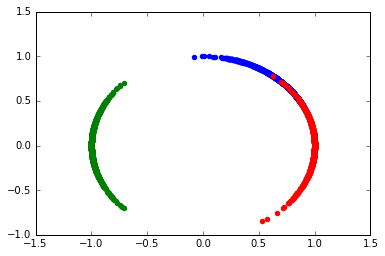
このようにすると24時付近のグループも1つの領域にまとまる。また、いかにも線形分離可能そうに見える。
再び機械学習を行ってみよう。
from sklearn import cross_validation

X = DataFrame({'cos': pd.concat(coss), 'sin': pd.concat(sins)})
y = pd.concat([Series([hour for _ in range(0, num_samples)]) for hour in hours])

X_train, X_test, y_train, y_test = cross_validation.train_test_split(X, y)
from sklearn.linear_model.perceptron import Perceptron
clf = Perceptron()
clf.fit(X_train, y_train)
clf.score(X_test, y_test)
0.94266666666666665
from sklearn.svm import LinearSVC
clf = LinearSVC().fit(X_train, y_train)
clf.score(X_test, y_test)
0.93733333333333335
from sklearn.svm import SVC
clf = SVC().fit(X_train, y_train)
clf.score(X_test, y_test)
0.93733333333333335
from sklearn.tree import DecisionTreeClassifier
clf = DecisionTreeClassifier().fit(X_train, y_train)
clf.score(X_test, y_test)
0.93066666666666664
線形分類器でも高い正答率を出すことができた。
Processingでフォントのアウトラインを読み取って再構築する
この記事ではProcessingでフォントのアウトライン(輪郭)をデータとして取得し、 そのデータを元にいくつかの仕方で再構築する方法を試していく。
フォントのアウトラインを読み取る
フォントのアウトラインを取得するためのProcessing独自の関数といったものは存在しないようだ。 JavaのAWTではFontからGlyphVectorを取得し、getOutlineメソッドでアウトラインを取得することができるのでこれを使用する。
import java.awt.Font;
import java.awt.font.FontRenderContext;
import java.awt.image.BufferedImage;
import java.awt.geom.PathIterator;

PathIterator createOutline(String name, int size, String text, float x, float y) {
  FontRenderContext frc =
    new BufferedImage(1, 1, BufferedImage.TYPE_INT_ARGB)
      .createGraphics()
      .getFontRenderContext();

  Font font = new Font(name, Font.PLAIN, size);

  PathIterator iter = font.createGlyphVector(frc, text)
    .getOutline(x, y)
    .getPathIterator(null);

  return iter;
}
このメソッドでは最終的にPathIteratorというオブジェクトが得られる。 これはタートルグラフィックのように点から点をつなぐ情報を表現している。 これを使ってそのまま輪郭を描くには次のようにすればいい。
void drawNormally() {
  PathIterator iter = createOutline("Segoe UI", 50, "wonderful cool something", 10, 40);
  float coords[] = new float[6];
  while (!iter.isDone()) {
    int type = iter.currentSegment(coords);
    switch (type) {
      case PathIterator.SEG_MOVETO: // beginning of new path
        beginShape();
        vertex(coords[0], coords[1]);
        break;
      case PathIterator.SEG_LINETO:
        vertex(coords[0], coords[1]);
        break;
      case PathIterator.SEG_CLOSE: // back to last MOVETO point.
        endShape();
        break;
      case PathIterator.SEG_QUADTO:
        quadraticVertex(coords[0], coords[1], coords[2], coords[3]);
        break;
      case PathIterator.SEG_CUBICTO:
        bezierVertex(coords[0], coords[1], coords[2], coords[3], coords[4], coords[5]);
        break;
      default:
        throw new RuntimeException("should not reach here");
    }
    iter.next();
  }
}
結果は次のようになる。

再構築する
しかしこれだけだと回りくどい方法で画面に文字を描いたにすぎない。 低レベルに降りることによって、間違った方法で文字描画を再構築することが可能になる。
一筆書きにする
先のコードではSEG_MOVETOは線を引かずに位置を移動すること、SEG_CLOSEは図形の描画を一段落させることに対応していた。 この2つの役割を無視すると一筆書きのように線をつなぐようになる。
void draw2() {
  PathIterator iter = createOutline("Segoe UI", 50, "wonderful cool something", 10, 40);
  float coords[] = new float[6];
  beginShape();
  while (!iter.isDone()) {
    int type = iter.currentSegment(coords);
    switch (type) {
      case PathIterator.SEG_MOVETO:
        vertex(coords[0], coords[1]);
        break;
      case PathIterator.SEG_LINETO:
        vertex(coords[0], coords[1]);
        break;
      case PathIterator.SEG_CLOSE:
        break;
      case PathIterator.SEG_QUADTO:
        quadraticVertex(coords[0], coords[1], coords[2], coords[3]);
        break;
      case PathIterator.SEG_CUBICTO:
        bezierVertex(coords[0], coords[1], coords[2], coords[3], coords[4], coords[5]);
        break;
      default:
        throw new RuntimeException("should not reach here");
    }
    iter.next();
  }
  endShape();
}
結果は次のようになる。

曲線と直線を分離する
少し物足りないので今度は直線を表す移動と曲線を表す移動を別々に一筆書きしてみる。
void draw3() {
  stroke(#ff4a5d);

  PathIterator iter = createOutline("Segoe UI", 50, "wonderful cool something", 10, 40);
  float coords[] = new float[6];
  beginShape();
  boolean init = true;
  while (!iter.isDone()) {
    int type = iter.currentSegment(coords);
    switch (type) {
      case PathIterator.SEG_MOVETO:
        if (init) vertex(coords[0], coords[1]);
        init = false;
        break;
      case PathIterator.SEG_LINETO:
      case PathIterator.SEG_CLOSE:
        break;
      case PathIterator.SEG_QUADTO:
        quadraticVertex(coords[0], coords[1], coords[2], coords[3]);
        break;
      case PathIterator.SEG_CUBICTO:
        bezierVertex(coords[0], coords[1], coords[2], coords[3], coords[4], coords[5]);
        break;
      default:
        throw new RuntimeException("should not reach here");
    }
    iter.next();
  }
  endShape();
}

void draw4() {
  stroke(#6144b0);

  PathIterator iter = createOutline("Segoe UI", 50, "wonderful cool something", 10, 40);
  float coords[] = new float[6];
  beginShape();
  boolean init = true;
  while (!iter.isDone()) {
    int type = iter.currentSegment(coords);
    switch (type) {
      case PathIterator.SEG_MOVETO:
        if (init) vertex(coords[0], coords[1]);
        init = false;
        break;
      case PathIterator.SEG_LINETO:
        vertex(coords[0], coords[1]);
        break;
      case PathIterator.SEG_CLOSE:
      case PathIterator.SEG_QUADTO:
      case PathIterator.SEG_CUBICTO:
        break;
      default:
        throw new RuntimeException("should not reach here");
    }
    iter.next();
  }
  endShape();
}
結果は次のようになる。おもしろい効果が得られるようになってきた。


手書き風にする
一筆書きなのでもう少し手書き風にすることを考える。
Processing用のライブラリとしてHandyというものがあるのでこれを利用する。 使い方はHandyRendererというオブジェクトを作成して、Processingの組み込みのbeginShapeやvertexの代わりにそのオブジェクトの同名メソッドを呼べばよい。
HandyRenderer h;

void setup() {
  size(640, 60);
  smooth();
  h = new HandyRenderer(this);
  noLoop();
}

void drawHandy() {
  noFill();
  stroke(#6144b0);

  PathIterator iter = createOutline("Segoe UI", 50, "wonderful cool something", 10, 40);
  float coords[] = new float[6];
  h.beginShape();
  boolean init = true;
  while (!iter.isDone()) {
    int type = iter.currentSegment(coords);
    switch (type) {
      case PathIterator.SEG_MOVETO:
        if (init) h.vertex(coords[0], coords[1]);
        init = false;
        break;
      case PathIterator.SEG_LINETO:
        h.vertex(coords[0], coords[1]);
        break;
      case PathIterator.SEG_CLOSE:
      case PathIterator.SEG_QUADTO:
      case PathIterator.SEG_CUBICTO:
        break;
      default:
        throw new RuntimeException("should not reach here");
    }
    iter.next();
  }
  h.endShape();
}

曲線のパスだけ塗りつぶす
やっぱり手書きはやめて曲線の部分だけ塗りつぶすことにする。
void drawCurveClosed() {
  fill(#ff4a5d);
  stroke(#ff4a5d);
  PathIterator iter = createOutline("Segoe UI", 50, "wonderful cool something", 10, 40);
  float coords[] = new float[6];
  while (!iter.isDone()) {
    int type = iter.currentSegment(coords);
    switch (type) {
      case PathIterator.SEG_MOVETO: // beginning of new path
        beginShape();
        vertex(coords[0], coords[1]);
        break;
      case PathIterator.SEG_LINETO:
        //vertex(coords[0], coords[1]);
        break;
      case PathIterator.SEG_CLOSE: // back to last MOVETO point.
        endShape();
        break;
      case PathIterator.SEG_QUADTO:
        quadraticVertex(coords[0], coords[1], coords[2], coords[3]);
        break;
      case PathIterator.SEG_CUBICTO:
        bezierVertex(coords[0], coords[1], coords[2], coords[3], coords[4], coords[5]);
        break;
      default:
        throw new RuntimeException("should not reach here");
    }
    iter.next();
  }
}

この記事のコードの全体はGistに置いた。